Merge CSV headers in R
Usually when you work with data from Public Data Services like INE (Spanish Statistical Office) you have to deal with a Excel files with a non usable format: metadata in the first rows, notes at the bottom, empty columns, empty rows, etc. You have to do a small data processing in order to start working.
Everyone knows the benefits of the CSV format, but precisely these metadata are there for one reason: unlike CSV where we only have the data itself, if we open this file within a few months this metadata will let you know exactly what data it contains or where it comes from. For this reason, I think that sometimes it is not a bad idea that the first phase of working with data is reading directly from an Excel format (instead of CSV).
For these cases I usually use R due to its reproducible workflow and of course because of the whole universe of packages, specially Tidyverse, an opinionated collection of R packages designed for data science.
Well, days ago I had to deal with a dataset that had a format with a problem I didn’t face before, it had a double header like the ones shown in the following picture:
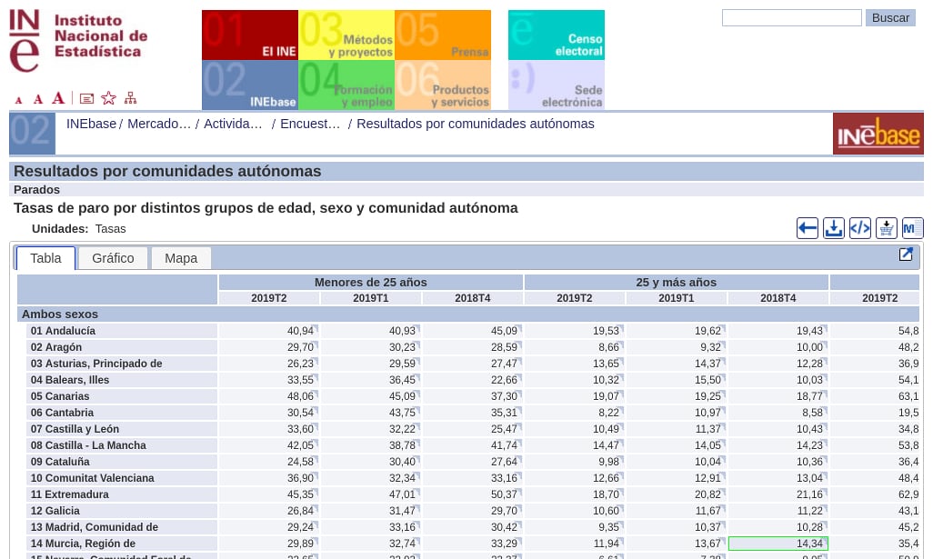 Capture from the Spanish Statistical Office site. Unemployment rate by ages and year quarters.
I spent hours searching the web looking for a solution but I didn’t find any. I finally opted for create a function to clean this dataset. My goal was to merge both rows and ended up with a column names as Menores de 25 años_2019T2, Menores de 25 años_2019T1 or Menores de 25 años_2018T4, i.e. combine the two rows with an underscore. I will show step by step a case in which this function could be used. If you prefer, you can go directly to the full script. First of all, I read a xlsx file with the amazing read_xlsx from Tidyverse and skip the first 6 lines.
library(tidyverse)
library(ggplot2)
library(janitor)
library(readxl)

filePath <- "data/4247.xlsx"

csv <- read_xlsx(filePath, skip = 6)
The function itself:
# This function fills empty cells with previous values to the right and then combine them with the row above
combineHeaders <- function(data){

  # store the row
  row <- colnames(data)

  # Get unique values, the ones will be repeated
  types <- row[is.na(as.numeric(gsub("\\.", "", row)))]

  # Create an index that will be incremented across the vector 'types'
  z <- 1

  # Store the first as the default one
  type <- types[z]

  # Iterate through colnames
  for(i in 1:length(row)){
    variable <- row[i]

    # Assume the work starts at the second column
    if (i!=1) {
      # combine with the previous row
      row[i] <- paste(type, data[1, ][i], sep = "_")

      # If current value is equal to the second one from unique values it updates the default value
      if (z + 1 <= length(types) & variable == types[z + 1]) {
        z <- z + 1
        type <- types[z]
        row[i] <- paste(type, data[1, ][i], sep = "_")
      }
    }

  }
  return(row)
}
I am completely sure that there must be a cleaner way or an R package that solves this problem but I have been unable to find it. Basically, what combineHeaders does is to store in the variable types those column names of the first row in a vector (discarding those column names that are numbers, as R / RStudio puts by default). Then iterates through all the column names in the first row (the original one from which we have extracted types), creates a default index (variable z) initialized to 1 and creates a variable called type that points to the first element of types through z value. In this iteration, it assigns the first element of the types vector (the value of the type) to the first elements. If a column name is equal to the next types element, it increases the value of z by one and updates type.
Then I assign the vector result of the funcion as the new csv header and apply some dplyr’s magic pipes for cleaning the data, renaming the first column and create a couple of variables from the first column.
# Assign the new headers from combineHeaders
names(csv) <- combineHeaders(csv)

cleaned <- csv %>%
  remove_empty('cols') %>%
  remove_empty('rows') %>%
  slice(3:19) %>%
  rename(
    ccaa = 1
  ) %>%
  mutate(
    id = substr(ccaa, 0, 2),
    ccaa = substring(ccaa, 3)
  ) %>%
  select(id, everything(), -matches("Menores de 25 años"), -matches("25 y más años"))
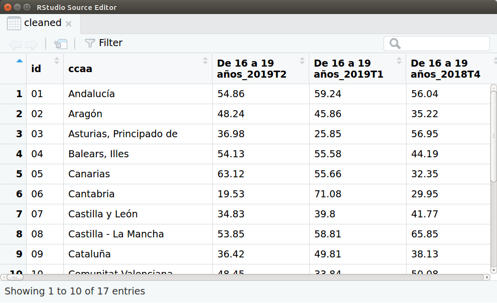 Capture of the data-frame ‘cleaned’.
Then I convert all the data-frame to long format, divide the previous headers into two new variables using separate and parse temporal variables to a date format:
tidied_data <- gather(cleaned, group, value, 3:length(colnames(cleaned))) %>%
  separate(group, c('group', 'quarter'), sep = '_') %>%
  mutate(
    value = as.numeric(value),
    date = as.Date(paste(substring(quarter, 1, 4), as.integer(substring(quarter, 6, 7)) * 3, 1, sep = "-"))
  )
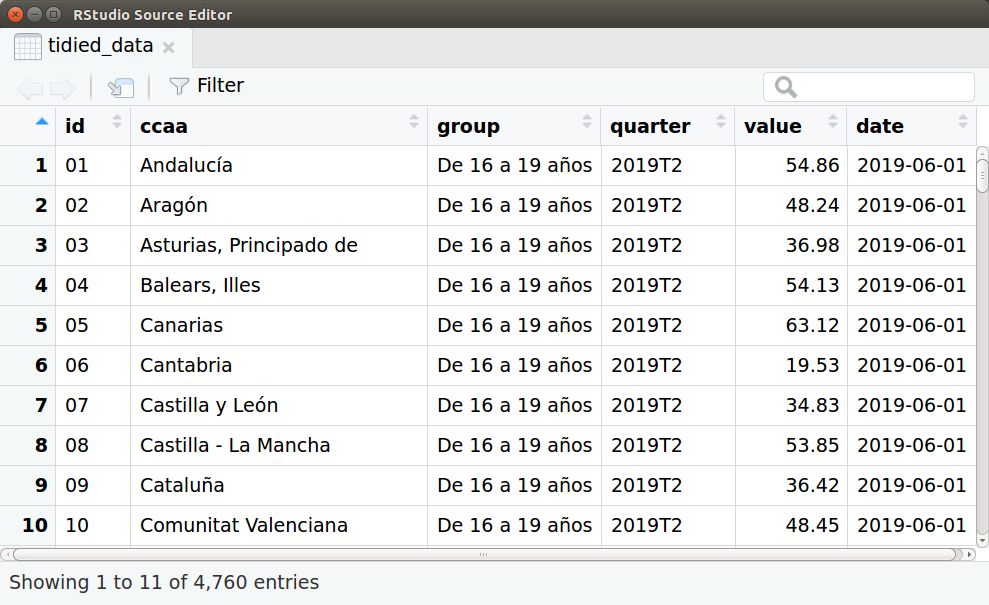 Capture of the data-frame ‘tidied_data’.
And finally a plot using ggplot. The code:
ggplot(data=tidied_data, aes(x = date, y = value)) +
  geom_line(aes(color = group)) +
  scale_color_manual(values = c("#966bff", "#FF6AD5", "#ffde8b", "#20de8b")) + # Color scale by vapeplot
  facet_wrap( ~ ccaa, ncol = 4) +
  ggtitle("Unemployment rates by age groups and regions") +
  theme_minimal() +
  theme(axis.title.x=element_blank(),
        axis.ticks.x=element_blank(),
        axis.title.y=element_blank(),
        axis.ticks.y=element_blank(),
        plot.margin = unit(c(0.5,0.5,0.5,0.5), "cm"))
And the result:
